
Conditional Variational Auto-Encoders are a tool for modeling $p(y|x)$. Variational Auto-Encoders allow us to generate new samples, that look like they come from the training dataset. CVAEs take this a step further and allow us to generate samples that also satisfy a specified condition.
In practice, this allows us to do things like generate specific digits that look like they come from MNIST.
Interactive Example
Enter a number of your choice and have a pre-trained cvae generate it as hand-written digits. This demo runs in your browser and may be slower on old devices. Getting bad results? Please note that the learned model parameters are rounded aggressively to improve page-load performance.
So, how does this work? I will explain the mathematical reasoning behind the algorithm first. Then I will outline how the mathematics can be translated into code, using Python and PyTorch. If you want to jump straight into the code, you can have a look at the GitHub repository for this article.
Auto-Encoding Variational Bayes
Let's start out by asking the following question: How can we model the distribution $p(y)$?
We start by assuming that we are given a dataset $ \mathcal{D} = \{y^{(i)}\}^N_{i=1} $ with independent and identically distributed (i.i.d.) samples. To make the problem tractable, we will also assume that the random process which produces the dataset involves a random latent variable $z$, with a known distribution $p(z)$. (This latent variable is why the method is called auto-encoding variational Bayes.)
Additionally assuming we have a parameterized distribution $p_{\theta}(y|z)$, we can now state our training objective: We want to maximize
$$ \log p_{\theta}(\mathcal{D}) = \log p_{\theta}(y^{(1)}, \ldots, y^{(N)}) = \sum_{i=1}^N \log p_{\theta}(y^{(i)}), $$
where $ p_{\theta}(y^{(i)}) = \int_z p_{\theta}(y|z) p(z) \text{d}z $, w.r.t. (with respect to) $ \theta $. That is, we want to maximize the log-probability of the dataset given our model distribution.
Conceptually, there is no difficulty here. However, in practice, marginalizing $z$ (computing the integral) is far to expensive for any interesting problem. The key insight that allows us to deal with this, is recognizing that for most $z$ we will get: $p(y|z) \approx 0$. So instead of integrating over all $z$, we could just focus on those that are likely to produce the desired $y$.
Since we don't know which $z$ are likely to give a valid $y$, we introduce a second parameterized distribution: $ q_{\theta}(z|y) $. We will use this distribution to approximate $p(z|y)$ during training.
Recap
So far we introduced a few functions we want to learn, as well as functions we know or care about. They are:
- $ p(y) $ - The function we want to model.
- $ p(z) $ - A function we assume we know. (In practice, we usually choose a Gaussian with unit variance.)
- $ p_{\theta}(y|z) $ - The function we want to learn. Since we know $p(z)$, this gives us $p(y)$.
- $ p(z|y) $ - A function we would like to know but don't know. Knowing it would help with training.
- $ q_{\theta}(z|y) $ - A function we can use to approximate $p(z|y)$.
Notice that we have to choose a parametric form for the functions we want to learn. So we know $ p_{\theta}(y|z) $ and $ q_{\theta}(z|y) $, but not the correct $ \theta $.
Now we can take this mess of functions and apply some statistics to tidy it up. To this end let me introduce the:
Kullback-Leiber Divergence
The KL-Divergence measures the difference between two distributions and is defined as:
$$ \mathcal{D}_{KL}[P(A)||Q(A)] = - \mathbb{E}_{A \sim P(A)}[\log\frac{Q(A)}{P(A)}] = \sum_i P(A_i) \log\frac{P(A_i)}{Q(A_i)}. $$
An important property of the KL-Divergence is that it is always non-negative. Now we have all the tools we need to find a lower bound on $ \log p_{\theta}(\mathcal{D}) $.
The Variational Lower Bound
We start by applying Bayes Law, which tells us that $p(z|y) = p(y|z) \frac{p(z)}{p(y)} $, to:
$$ \mathcal{D}_{KL}[q_{\theta}(z|y)||p(z|y)] = \\ \mathbb{E}_{z \sim q_{\theta}(z|y)}[\log q_{\theta}(z|y) - \log p_{\theta}(y|z) - \log p(z) + \log p(y)]. $$
Rearranging the whole thing a bit, and moving the $ \log p(y) $ term out of the expectation, as it has no dependence on $ z $, we get:
$$ \log p(y) - \mathcal{D}_{KL}[q_{\theta}(z|y)||p(z|y)] = \\ \mathbb{E}_{z \sim q_{\theta}(z|y)}[\log p_{\theta}(y|z)] - \mathcal{D}_{KL}[q_{\theta}(z|y)||p(z)]. $$
Unless you are familiar with the KL-Divergence, this may not really look like progress. However, we already have (most of) the pieces to start writing some code.
Looking at the left-hand-side, we see our original objective, which is great. But we also see the KL-Divergence between our approximation $ q_{\theta}(z|y) $ and the true distribution $p(z|y)$, which means that by maximizing the left-hand-side, we will also obtain that approximation as an added bonus.
Since the KL-Divergence is always positive, the left-hand-side is a lower bound of $\log p(y)$. It is called the variational lower bound.
The right hand side now only contains quantities we know, so we can now perform optimization using a gradient based optimizer like SGD or Adam.
PyTorch Implementation of Variational Bayes
Now that we saw the maths, I will explain how to implement the method using Python and PyTorch. The full source code can be found in this GitHub repository. Here, I will only cover the model and the loss function.
Before we jump into the code, we need to make a few decisions. Earlier, we assumed we knew $ p(z) $ and had parametric functions for $ p_{\theta}(y|z) $ and $ q_{\theta}(z|y) $. Now we need to be a bit more concrete.
Since it's mathematically convenient and we can sample from it, we make the choice:
$$ p(z) = \mathcal{N}(z|\mu = 0, \sigma^2 = 1), $$
where $\mathcal{N}$ denotes the Normal or Gaussian distribution. As for the parametric distributions, we decide to use:
$$ p_{\theta}(y|z) = \mathcal{N}(y|\mu = f_{\theta}(z), \sigma^2 = 1) $$
and
$$ q_{\theta}(z|y) = \mathcal{N}(y|\mu = g_{\theta}(y), \sigma^2 = h_{\theta}(y)). $$
For the parametric functions $f_{\theta}$, $g_{\theta}$ and $h_{\theta}$, we use fully-connected neural networks with linear-rectifiers as our non-linearity. (Except for the last layer of $f_{\theta}$, which uses sigmoid).
Defining our Model
We start with defining these functions:
class Model(nn.Module):

    def __init__(self):
        super().__init__()

        self.encoder = nn.Sequential(
            nn.Linear(28**2, 512),
            nn.ReLU(),
            nn.Linear(512, 512),
            nn.ReLU()
        )

        self.mu = nn.Linear(512, 256)
        self.log_var = nn.Linear(512, 256)

        self.decoder = nn.Sequential(
            nn.Linear(256, 512),
            nn.ReLU(),
            nn.Linear(512, 512),
            nn.ReLU(),
            nn.Linear(512, 28**2),
            nn.Sigmoid()
        )

    ...
Our model looks a bit like an auto-encoder, which is why I choose to call the
functions encoder and decoder. decoder corresponds to $f_{\theta}$, while
we use weight-sharing for $g_{\theta}$ and $h_{\theta}$, so that
mu(encoder(y)) is $g_{\theta}$ and log_var(encoder(y)) is $\log
h_{\theta}(y)$.
Notice that we use the logarithm, as this will help with numeric stability.
Now we want to be able to train these parameters using stochastic gradients. To do this, we define the forward pass of our model:
class Model(nn.Module):

    ...

    def forward(self, x):
        # Find parameters for latent distribution
        h = self.encoder(x.view(-1, 28**2))
        mu = self.mu(h)
        z = mu

        if self.training:
            # Re-parametrization trick
            # (move sampling to input)
            log_var = self.log_var(h)
            eps = torch.randn_like(mu)
            z = eps.mul(log_var.mul(0.5).exp()).add_(mu)

        r = self.decoder(z).view(-1, 1, 28, 28)

        # Only return p(z|x) parameters if training
        if self.training:
            return (r, mu, log_var)
        return r
Notice that the variable we model is called x in the code, whereas we called
it $y$ when going through the mathematics.
This piece of code contains something very important: The re-parametrization trick. Our objective requires us to compute the expectation of $z \sim q_{\theta}(z|y)$. To improve performance, we will approximate this expectation by sampling from $q_{\theta}(z|y)$.
However, sampling from a random distribution is a non-differentiable process, which prevents us from using gradient based optimization methods. To get ourselves out of this one, we instead introduce a new random variable $\epsilon \sim \mathcal{N}(\epsilon|0,1)$. Rather than sampling $z$ directly, we find it as:
$$ z = \epsilon \times \sqrt{\sigma^2} + \mu = \epsilon \times \sqrt{h_{\theta}(y)} + g_{\theta}(y) $$
This re-parametrization effectively moves the sampling operation to the input, which means that we can once more compute gradients w.r.t all parameters.
Defining the loss function
The second thing we need to give PyTorch so that we can train our model is a loss function. Since we want to maximize our objective w.r.t. our parameters, the loss function will be the negative of the objective:
$$ \mathcal{D}_{KL}[q_{\theta}(z|y)||p(z)] - \mathbb{E}_{z \sim q_{\theta}(z|y)}[\log p_{\theta}(y|z)] \approx \mathcal{D}_{KL}[q_{\theta}(z|y)||p(z)] - \log p_{\theta}(y|z) $$
Written using PyTorch, this becomes:
def loss_fn(x, r, mu, log_var):
    # Reconstruction loss
    loss_r = F.binary_cross_entropy(r, x, reduction="sum")
    # KL Divergence
    loss_kl = - 0.5 * (1 + log_var - mu**2 - log_var.exp()).sum()
    return loss_r + loss_kl
Notice that x is $y$ and r is $f\{\theta}$, while mu and log_var are
the parameters of the distribution $p_{\theta}(z|y)$._
The KL-Divergence term is easy to explain: It is simply the analytic solution, given our choice of distributions. (See the appendix of Auto-Encoding Variational Bayes for a derivation.)
For the $\log p_{\theta}(y|z)$ term (reconstruction loss), the choice of loss is motivated as follows: We know that, since our distribution is Gaussian, its mode (maximum) is at $y=\mu$ (the expectation). So we maximize the probability of $y$ iff (if and only if) $\mu = f_{\theta} = y$. In other words: We want $f_{\theta}$ to reproduce the original variable $y$. Instead of binary cross entropy, we could also have chosen something like mean square error. Any loss that is minimized for $f_{\theta} = y$ should work in principle.
The rest of the code simply loads MNIST and preforms a gradient based minimization of our loss using Adam.
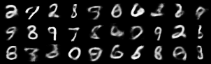
I encourage you, to download the code from GitHub and run the example
vae.py yourself, and try to play with it a bit. The results should look
something like this:
Conditional Variational Bayes
So far we can sample from $p(y) = p_{\theta}(y|z) p(z)$, but whenever we sample from this distribution, we get an image of a random digit. It would be much cooler, if we could also specify, which digit we want. (Like in the interactive example at the beginning.)
To do this, we need to model the conditional distribution $p(y|x)$, where $x$ represents the digit we want.
We will consider the case, where the latent variables $z$ are independent from the input variables $x$, since this case will allow us to use the same loss function as before.
Functions of interest
As before, there are a few functions we need to keep in mind:
- $ p(y|x) $ - The function we want to model.
- $ p(z) $ - A function we assume we know. (This is the same as before.)
- $ p_{\theta}(y|z,x) $ - The function we want to learn. Since we know $p(z)$, this gives us $p(y).$
- $ p(z|y,x) $ - A function we would like to know but don't know. Knowing it would help with training.
- $ q_{\theta}(z|y,x) $ - A function we can use to approximate $p(z|y,x).$
The (New) Variational Lower Bound
In complete analogy to before we use Bayes theorem, which tells us that $p(z|y,x) = p(y|z,x) \frac{p(z)}{p(y|x)} $. Using the same procedure as for the not conditioned case, we finally obtain:
$$ \log p(y|x) - \mathcal{D}_{KL}[q_{\theta}(z|y,x)||p(z|y,x)] =\\ \mathbb{E}_{z \sim q_{\theta}(z|y,x)}[\log p_{\theta}(y|z,x)] - \mathcal{D}_{KL}[q_{\theta}(z|y,x)||p(z)]. $$
Changes to the Code
When it comes to implementing this condition model in PyTorch, we can basically
almost copy our previous code. The only change we need to make is to include $x$
as the input in both our encoder and decoder. To this end, we amend them as
follows:
...

self.encoder = nn.Sequential(
    nn.Linear(28**2 + 10, 512),
    nn.ReLU(),
    nn.Linear(512, 512),
    nn.ReLU()
)

...

self.decoder = nn.Sequential(
    nn.Linear(256 + 10, 512),
    nn.ReLU(),
    nn.Linear(512, 512),
    nn.ReLU(),
    nn.Linear(512, 28**2),
    nn.Sigmoid()
)

...
We will be passing $x$ by concatenating the previous input with a vector which is given by:
$$ \vec{x}_i = \{^{1,\text{ }i = \text{number}}_{0,\text{ otherwise}}. $$
We can interpret this vector as given the probability that $y$ is the respective number.
As before, you should have a look at the code on GitHub to see all the
adjustments we need to make in the conditioned case. You can also run the
example cvae.py to see the training process. The interactive example at the
beginning of the article was trained using this model.
References - Read the Papers
These papers are where all of the above ideas originate. If you want to dive deeper, you should read some of them.